SIG con R: Vectores part 1

SIG

Apuntes de la escuela ambiental

Author

Daniela O

Published

July 27, 2024

Sistemas de información geográfico con R

Cargar y trazar archivos Shapefile

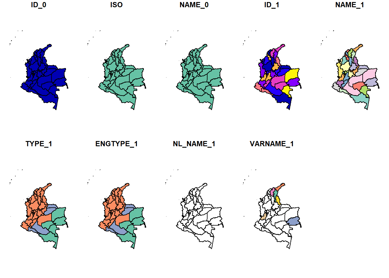
library(sf) # para abrir archivos shp
library(sp) 
# library(rgdal)

# leyendo shapefile de Colombia
1col_admin<- read_sf("COL_adm/COL_adm1.shp")
2plot(col_admin)

1: código de library sf, te visualiza el shp como base de datos
2: Se generan varios mapas que corresponden al número de columnas de la base de datos.

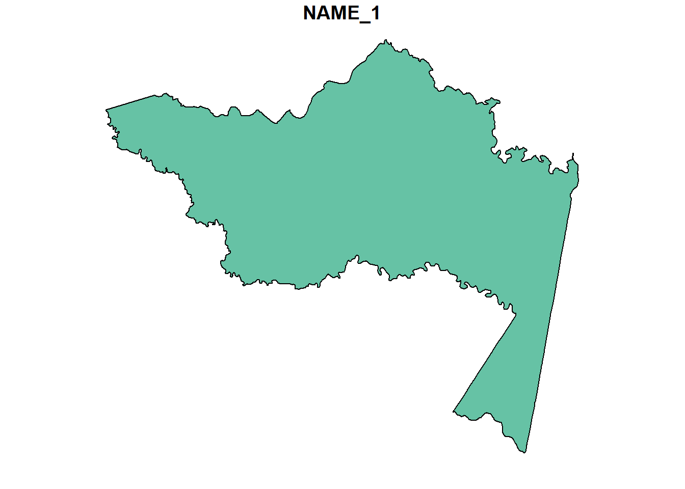
plot(col_admin[1,5]) # especificando la fila y la columna

# codigo del paquete rgdal 
# col_admin2<- readOGR("COL_adm/COL_adm1.shp")

Dibujar geometrías vectoriales

Crear geometrías vectoriales

#install.packages("mapedit")
#install.packages("mapview")
library(mapview)
library(mapedit)
library(dplyr)

# 1. Cargar una ventana con un mapa base
mapview()

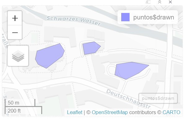
# para colocar puntos, poligonos o lineas
1 puntos<- mapview() |> editMap()

1: Esto te abre un panel de herramientas para colocar puntos y polígonos dentro del mapa interactivo y se guarda como base de datos

# Guardando como archivo shape
library(sf)
mapview(puntos$drawn) # se selecciona todo lo que se dibujo anteriormente

NULL

# write_sf(puntos$drawn, "COL_adm/puntos.shp") 
# solo se pueden guardar o solo puntos, poligonos, no se pueden mezclar.

Convertir csv a forma / manipulación vectorial

library(tidyverse)
library(sf)
library(mapview)

# abriendo base de datos 
obs<- read.csv2("specie_rana.csv", header = TRUE)
head(obs)

                     Species Longitude Latitude Temp Prec Prec_qs Prec_qh
1 Leucostethus fraterdanieli  -75.8531   4.8668  223 1756     678     299
2 Leucostethus fraterdanieli  -75.8348   4.6978  217 1870     647     316
3 Leucostethus fraterdanieli  -75.5791   4.7352  177 2079     801     313
4 Leucostethus fraterdanieli  -75.8320   4.6083  217 1762     652     271
5 Leucostethus fraterdanieli  -75.4441   5.1852  159 2292     991     342
6 Leucostethus fraterdanieli  -75.6869   5.2415  233 1852     677     287
  elevacion
1       999
2      1162
3      1918
4      1155
5      2213
6       838

# convirtiendo a shp
obs_shp<- st_as_sf(obs, coords = c("Longitude", "Latitude"), crs=4326)
head(obs_shp)

Simple feature collection with 6 features and 6 fields
Geometry type: POINT
Dimension:     XY
Bounding box:  xmin: -75.8531 ymin: 4.6083 xmax: -75.4441 ymax: 5.2415
Geodetic CRS:  WGS 84
                     Species Temp Prec Prec_qs Prec_qh elevacion
1 Leucostethus fraterdanieli  223 1756     678     299       999
2 Leucostethus fraterdanieli  217 1870     647     316      1162
3 Leucostethus fraterdanieli  177 2079     801     313      1918
4 Leucostethus fraterdanieli  217 1762     652     271      1155
5 Leucostethus fraterdanieli  159 2292     991     342      2213
6 Leucostethus fraterdanieli  233 1852     677     287       838
                 geometry
1 POINT (-75.8531 4.8668)
2 POINT (-75.8348 4.6978)
3 POINT (-75.5791 4.7352)
4  POINT (-75.832 4.6083)
5 POINT (-75.4441 5.1852)
6 POINT (-75.6869 5.2415)

mapview(obs_shp)

Luego esto se puede exportar como archivo shapefile como vimos anteriormente

Descargar formas de países en R

# Descargar paises desde R
library(raster) # paquete con shp de paises, wordclim y modelos de elevación 
library(sf)
library(dplyr)
library(mapview)
library(geodata) # version actual de library raster
library(terra)

#getData("ISO3")
#Mexico_2<-gadm(country="MEX", level= 2, path ="Mexico" ) |> st_as_sf()

#mapview(Mexico_2)

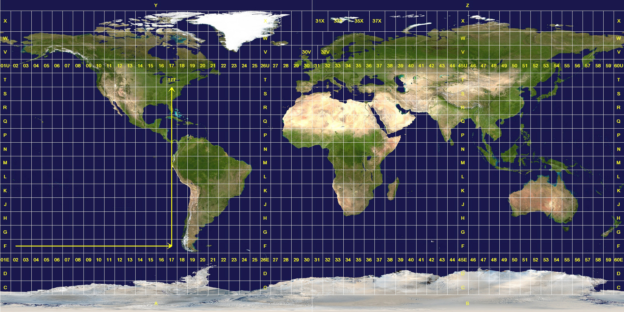
Cambiar el sistema de coordenadas de referencia de un shapefile 📍

Para cambiarlo nos dirigimos a la página: https://spatialreference.org/ para encontrar las diferentes proyecciones.

# Cambiar sistemas de coordenas de una geometria vectorial
library(sf)
library(raster)
library(geodata)

# obtener limite de un pais de interes que nos servir? como ejemplo

colombia<-gadm(country="COL", level= 0, path ="Colombia" ) |> st_as_sf()
colombia

Simple feature collection with 1 feature and 2 fields
Geometry type: MULTIPOLYGON
Dimension:     XY
Bounding box:  xmin: -81.84153 ymin: -4.228429 xmax: -66.83774 ymax: 15.91248
Geodetic CRS:  WGS 84
  GID_0  COUNTRY                       geometry
1   COL Colombia MULTIPOLYGON (((-69.92329 -...

# reproyectar con proj4
col_magna<- st_transform(colombia, "+proj=tmerc +lat_0=4.596200416666666 +lon_0=-74.07750791666666 +k=1 +x_0=1000000 +y_0=1000000 +ellps=GRS80 +towgs84=0,0,0,0,0,0,0 +units=m +no_defs")
col_magna

Simple feature collection with 1 feature and 2 fields
Geometry type: MULTIPOLYGON
Dimension:     XY
Bounding box:  xmin: 152612.3 ymin: 22983.61 xmax: 1807919 ymax: 2258249
Projected CRS: +proj=tmerc +lat_0=4.596200416666666 +lon_0=-74.07750791666666 +k=1 +x_0=1000000 +y_0=1000000 +ellps=GRS80 +towgs84=0,0,0,0,0,0,0 +units=m +no_defs
  GID_0  COUNTRY                       geometry
1   COL Colombia MULTIPOLYGON (((1461621 271...

Se busca en la página https://spatialreference.org/ el tipo de proyección (en este caso la Magma SIRGAS) y se pega el codigo que ofrece

# reproyectar con codigo EPSG
col_utm<-st_transform(colombia, crs= 32618)
col_utm

Simple feature collection with 1 feature and 2 fields
Geometry type: MULTIPOLYGON
Dimension:     XY
Bounding box:  xmin: -245935.3 ymin: -469204.3 xmax: 1411165 ymax: 1763314
Projected CRS: WGS 84 / UTM zone 18N
  GID_0  COUNTRY                       geometry
1   COL Colombia MULTIPOLYGON (((1064147 -46...