SIG con R: Vectores part 2

SIG

Apuntes de la escuela ambiental

Author

Daniela O

Published

July 28, 2024

Continuación de apuntes con manipulación y operación con vectores

Crear polígonos mínimos convexos

En ecología y biología nos ayuda para determinar hábitos hogareños, es decir, encontrar el área en el que se desplaza una especie.

# librerias requeridas
library(sf)
library(mapview)
library(dplyr)

# Cargamos el dataframe con los puntos

registros<-read.csv("Registros.csv", header = T) %>% st_as_sf(coords=c("Longitude","Latitude"), crs=4326)
mapview(registros)

# Observar solo la sp1
sp1<-filter(registros, Species=="sp1")
mapview(sp1)

# Generar PMC para una sola especie
pmc1<- sp1 %>% group_by(Species) %>%
    summarise(geometry= st_combine(geometry)) |> st_convex_hull()

mapview(list(pmc1, sp1))

# Generar poligonos para todas las especies
pmc_spp<- registros %>% group_by(Species) %>%
    summarise(geometry= st_combine(geometry)) %>%
    st_convex_hull()

mapview(list(pmc_spp, registros))

Crear polígonos alpha hull

#install.packages("alphahull")
#instalar maptools
#("maptools", repos = "https://packagemanager.posit.co/cran/2023-10-13")
library(maptools)
library(alphahull)
library(sp)
#library(rgdal)

# Funcion para convertir los a-hull en shp (https://stat.ethz.ch/pipermail/r-sig-geo/2012-March/014409.html)

ah2sp <- function(x, increment=360, rnd=10, proj4string=CRS(as.character(NA))){
    require(alphahull)
    require(maptools)
    if (class(x) != "ahull"){
        stop("x needs to be an ahull class object")
    }
    # Extract the edges from the ahull object as a dataframe
    xdf <- as.data.frame(x$arcs)
    # Remove all cases where the coordinates are all the same      
    xdf <- subset(xdf,xdf$r > 0)
    res <- NULL
    if (nrow(xdf) > 0){
        # Convert each arc to a line segment
        linesj <- list()
        prevx<-NULL
        prevy<-NULL
        j<-1
        for(i in 1:nrow(xdf)){
            rowi <- xdf[i,]
            v <- c(rowi$v.x, rowi$v.y)
            theta <- rowi$theta
            r <- rowi$r
            cc <- c(rowi$c1, rowi$c2)
            # Arcs need to be redefined as strings of points. Work out the number of       points to allocate in this arc segment.
            ipoints <- 2 + round(increment * (rowi$theta / 2),0)
            # Calculate coordinates from arc() description for ipoints along the arc.
            angles <- anglesArc(v, theta)
            seqang <- seq(angles[1], angles[2], length = ipoints)
            x <- round(cc[1] + r * cos(seqang),rnd)
            y <- round(cc[2] + r * sin(seqang),rnd)
            # Check for line segments that should be joined up and combine their coordinates
            if (is.null(prevx)){
                prevx<-x
                prevy<-y
            } else if (x[1] == round(prevx[length(prevx)],rnd) && y[1] == 
                       round(prevy[length(prevy)],rnd)){
                if (i == nrow(xdf)){
                    #We have got to the end of the dataset
                    prevx<-append(prevx,x[2:ipoints])
                    prevy<-append(prevy,y[2:ipoints])
                    prevx[length(prevx)]<-prevx[1]
                    prevy[length(prevy)]<-prevy[1]
                    coordsj<-cbind(prevx,prevy)
                    colnames(coordsj)<-NULL
                    # Build as Line and then Lines class
                    linej <- Line(coordsj)
                    linesj[[j]] <- Lines(linej, ID = as.character(j))
                } else {
                    prevx<-append(prevx,x[2:ipoints])
                    prevy<-append(prevy,y[2:ipoints])
                }
            } else {
                # We have got to the end of a set of lines, and there are several such     sets, so convert the whole of this one to a line segment and reset.
                prevx[length(prevx)]<-prevx[1]
                prevy[length(prevy)]<-prevy[1]
                coordsj<-cbind(prevx,prevy)
                colnames(coordsj)<-NULL
                # Build as Line and then Lines class
                linej <- Line(coordsj)
                linesj[[j]] <- Lines(linej, ID = as.character(j))
                j<-j+1
                prevx<-NULL
                prevy<-NULL
            }
        }
        # Promote to SpatialLines
        lspl <- SpatialLines(linesj)
        # Convert lines to polygons
        # Pull out Lines slot and check which lines have start and end points that are the same
        lns <- slot(lspl, "lines")
        polys <- sapply(lns, function(x) { 
            crds <- slot(slot(x, "Lines")[[1]], "coords")
            identical(crds[1, ], crds[nrow(crds), ])
        }) 
        # Select those that do and convert to SpatialPolygons
        polyssl <- lspl[polys]
        list_of_Lines <- slot(polyssl, "lines")
        sppolys <- SpatialPolygons(list(Polygons(lapply(list_of_Lines, function(x) 
        { Polygon(slot(slot(x, "Lines")[[1]], "coords")) }), ID = "1")), 
        proj4string=proj4string)
        # Create a set of ids in a dataframe, then promote to SpatialPolygonsDataFrame
        hid <- sapply(slot(sppolys, "polygons"), function(x) slot(x, "ID"))
        areas <- sapply(slot(sppolys, "polygons"), function(x) slot(x, "area"))
        df <- data.frame(hid,areas)
        names(df) <- c("HID","Area")
        rownames(df) <- df$HID
        res <- SpatialPolygonsDataFrame(sppolys, data=df)
        res <- res[which(res@data$Area > 0),]
    }  
    return(res)
}

puntos<- read.csv("Registros.csv", header=TRUE)
sp1<-puntos %>% filter(Species=="sp1")

Defino Alfa y creo el poligono (el valor de alfa debe variar segun los puntos). En los datos NO deben haber x, y duplicados, sino la funcion saca ERROR. Los datos ya deben estar limpios

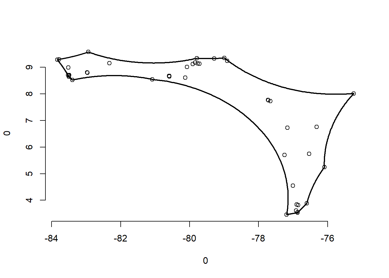
# Alfa hull
alpha=4.5 # ancho de poligono
1alfa_sp1<-ahull(x=sp1$Longitude, y=sp1$Latitude, alpha=alpha)
plot(alfa_sp1)

1: Comando del paquete alphahull

class(alfa_sp1)

[1] "ahull"

# transformo de ashape a spatial polygon
ob_shape<-ah2sp(alfa_sp1)
plot(ob_shape)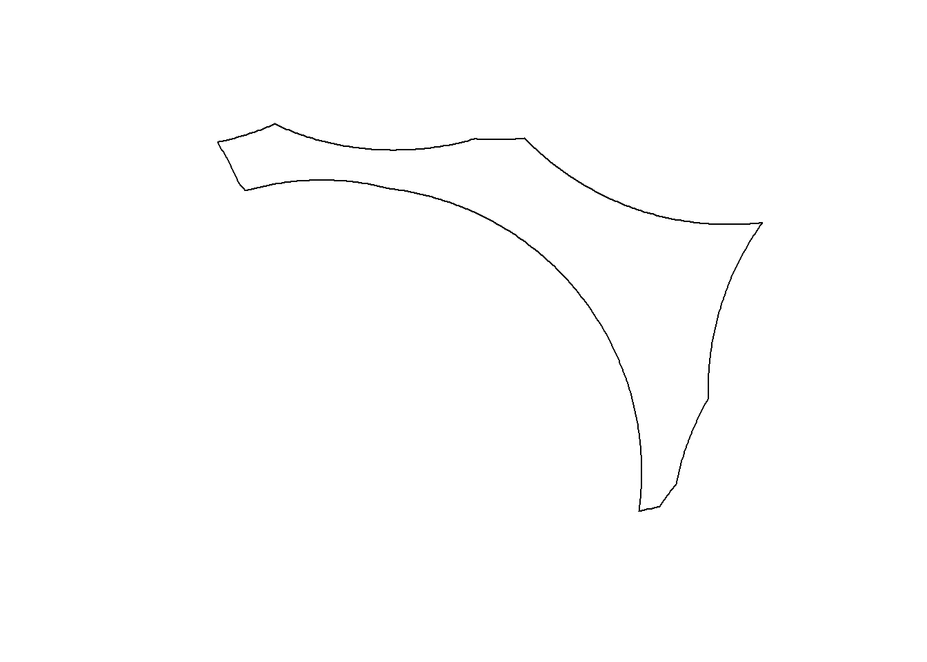

class(ob_shape)

[1] "SpatialPolygonsDataFrame"
attr(,"package")
[1] "sp"

# Exporto shape. Debo configurar el dsn.
# write_sf(obs_shp, "alpha_hull.shp")

Búferes

¿ Cómo dibujar un área sobre sobre un polígono ?

# librerias requeridas
library(sf)
library(mapedit)
library(mapview)
library(tidyverse)

# para dibujar los shapefile
poligono <-mapview() %>% editMap()
puntos <-mapview() %>% editMap()
lineas <-mapview() %>% editMap()

mapview(poligono$drawn)

#transformar sistemas de coordenadas
polig<- poligono$finished %>% st_transform(crs=32618)
point<- puntos$finished %>% st_transform(crs=32618)
rutas<- lineas$finished %>% st_transform(crs=32618)

mapview(list(polig, point, rutas))

# write_sf(poligono$drawn, "polig.shp")

Tengan en cuenta que el sistema de coordenadas de referencia nos marca las unidades de distancia (En este caso el sistema de coordenadas esta en UTM y trabaja las distancias en metros). Si quieren que las unidades sean metros deben reproyectar su capa. 1 km equivale a aproximadamente 0.0083333 grados

# creando buffer 
1polibuff<-st_buffer(polig, dist= 10000)
mapview(list(polig, polibuff))

puntbuff<-st_buffer(point, dist= 5000)
mapview(list(point, puntbuff))

linbuff<-st_buffer(rutas, dist= 500)
mapview(list(rutas, linbuff))

1: la distancia este en metros 😀 que equivalen a 10 km

# buffer negativo
polibuff2<-st_buffer(polig, dist= -10000)
mapview(list(polig, polibuff, polibuff2))

Calculando áreas

# Calculo de areas
1a_po<-st_area(polig)/1000000
a_pb<-st_area(polibuff)/1000000
a_pb2<-st_area(polibuff2)/1000000

1: Se divide entre un millón para pasar de \(m^2\) a \(km^2\)

areakm2<-c(a_po, a_pb, a_pb2)
# calculando diferencias entre los poligonos
areakm2[1]-areakm2[2]
areakm2[1]-areakm2[3]

col<- read_sf("COL_adm1.shp")
area_col<-st_area(col)/1000000

#calculo de areas de departamentos 
areas_depa<- col %>% mutate(AREAKM=st_area(col)/1000000)